While working with Excel you might have by mistake entered a formula which result in an error which says a circular reference identified. This is sometimes easier to fix and sometimes it get tricky to find and fix the error. In this post we will discuss in brief about the circular reference warning and solutions.
we will discuss
- What is Circular reference warning
- How to avoid the circular warning error
- Finding the circular reference error
- False flag for circular reference
- How to turn off the excel circular reference warning
What is circular reference warning?
A circular reference warning in Microsoft Excel is a warning message that appears when a formula in a cell refers back to itself or to a set of cells that eventually refer back to the original cell. This creates a circular loop in the calculation, and Excel cannot determine the final result.
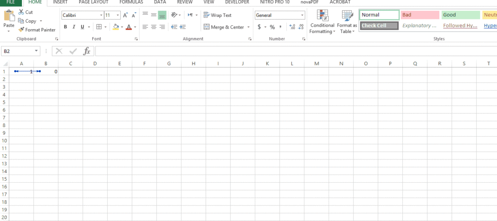
For example, consider the following scenario: Cell A1 contains the formula =B1+1, and Cell A2 contains the formula =A1+1. This creates a circular reference, because each cell refers back to the other, creating a loop that Excel cannot resolve.

When a circular reference is detected, Excel will usually show a warning message and will not complete the calculation. This is to prevent incorrect results and to avoid slowing down the performance of Excel.
To resolve a circular reference warning, you can either change the formula or modify the data to break the circular loop. In some cases, you can also use the =IF function to control the calculation and avoid the circular reference. It’s important to be careful when working with circular references, as they can cause unexpected results and can make it difficult to understand the calculation logic.
How to avoid circular reference error
Circular reference errors occur when a formula refers back to the cell that contains the formula, creating a loop that Excel cannot resolve. To avoid circular reference errors, you can follow these steps:
- Plan your calculation: Before you start entering formulas, think about the calculation logic and make sure it is structured in a way that avoids circular references.
- Use intermediate cells: Instead of referring directly from one cell to another, use intermediate cells to break the circular loop. For example, if Cell A1 refers to Cell A2 and Cell A2 refers to Cell A1, you can add a third cell, Cell A3, that calculates the intermediate result.
- Use the =IF function: You can use the =IF function to control the calculation and avoid circular references. For example, you can use the =IF function to only perform the calculation when a certain condition is met.
- Check your formulas: Regularly check your formulas and make sure that they are not referring back to themselves or to a set of cells that eventually refer back to the original cell.
By following these steps, you can avoid circular reference errors and ensure that your calculations are accurate and reliable. If you do encounter a circular reference error, make sure to resolve it as soon as possible to prevent incorrect results and slow performance.
How to find circular reference warning
Circular reference in Microsoft Excel, will make the excel sheet slow and sometimes it gets hangs. It is better to find the errors and correct them as soon as possible. You can use the following steps to check and rectify the error:
- Click the “Formulas” tab in the ribbon.
- In the “Formulas” tab, click on the “Error Checking” button in the “Formula Auditing” group.
- In the “Error Checking” dialog box, select “Circular References.”
- Excel will display a list of cells with circular references in the workbook.
- To see the cells that are involved in the circular reference, click on the cell in the list. Excel will highlight the cells involved in the circular reference and will display a warning message indicating that a circular reference has been detected.
- To resolve the circular reference, you can either change the formula or modify the data to break the circular loop.

Sometimes even after you figure out the error and rectify you will get the false flag of the error. Let’s see why it triggers false error and how to get it done.
You can also check out our other post to get the most useful excel shortcuts to help you in advancement.
False reference warning
A false circular reference warning occurs in Microsoft Excel when Excel displays a warning message for a circular reference, even though there is no actual circular reference in the calculation. This can happen if Excel’s calculation engine is not able to correctly determine the calculation logic, or if there is a problem with the formula.
To resolve a false circular reference warning, you can try the following steps:
- Check the formula: Make sure that the formula is correct and that it does not refer back to the cell that contains the formula or to a set of cells that eventually refer back to the original cell.
- Disable iterative calculation: If the false circular reference warning is due to iterative calculation, you can turn off iterative calculation by going to
“File” –> “Options” –> “Formulas” –> “Calculation options” and unchecking “Enable iterative calculation.”
- Remove any volatile functions: If the false circular reference warning is caused by a volatile function, such as =NOW() or =RAND(), remove the volatile function from the calculation.
- Refresh the workbook: If the false circular reference warning is due to a temporary problem with Excel, you can try refreshing the workbook by clicking the “Calculate Now” button in the “Formulas” tab in the ribbon.
By following these steps, you can resolve false circular reference warnings in Microsoft Excel, ensuring that your calculations are accurate and reliable. If the problem persists, you may need to seek assistance from Microsoft support or from a technical expert.
Excel circular reference warning turn off
To turn off the circular reference warning in Microsoft Excel, you can change the calculation options for your workbook. Here’s how:
- Select “File” tab and go to “Options.”
- In the “Excel Options” dialog box, select “Formulas.”
- Under “Calculation options,” uncheck the box next to “Enable iterative calculation.”
- Click “OK” to save the changes and close the dialog box.
With this option turned off, Excel will not display a warning message for circular references, but it will also not prevent circular references from occurring. Be aware that circular references can lead to incorrect results and slow down the performance of Excel, so it’s important to understand how they work and how to avoid them.

If you need to use circular references in your calculation, you can also control the number of iterations that Excel performs when calculating a circular reference. To do this, you can adjust the “Maximum Iterations” and “Maximum Change” options in the “Formulas” section of the “Excel Options” dialog box. However, be cautious when using these options, as they can affect the accuracy of the calculation and may cause unexpected results.
Conclusion:
Here we try to put some brief idea about the error, have you ever come across this error or warning what was the use case please let us know below in comments your experience. Also, if you need to add anything more or need us to correct anything please let us know. You can also leave a comment on our facebook page


